How We Reduced Painting Detection False Positives by 90%

47 false alerts per 8-hour shift. That was ProxControl's painting detection system after Phase 1. Technically accurate - the algorithm detected velocity drift correctly - but practically useless. Operators ignored every alert because most of them were triggered by normal painting behavior: pausing to reload, changing direction at edges, adjusting grip.

After Phase 2, false alerts dropped to 4 per shift. A 91% reduction. The core algorithm didn't change. Everything we did was about deciding when not to trigger an alert.

Key Takeaways > - Accuracy and usefulness are different problems. A 99% accurate system with 50 false positives per day is useless. > - Three techniques reduced our false positives by 91%: hysteresis thresholds, debounce windows, and movement gating. > - The hardest part wasn't the math. It was defining what "normal" painting behavior looks like from sensor data alone.

The Problem: Accurate But Useless

ProxControl builds industrial spray-painting systems for manufacturing lines. Their operators paint surfaces using robotic arms, and coating consistency matters. Too fast, the coating is thin and fails quality checks. Too slow, it drips and wastes material.

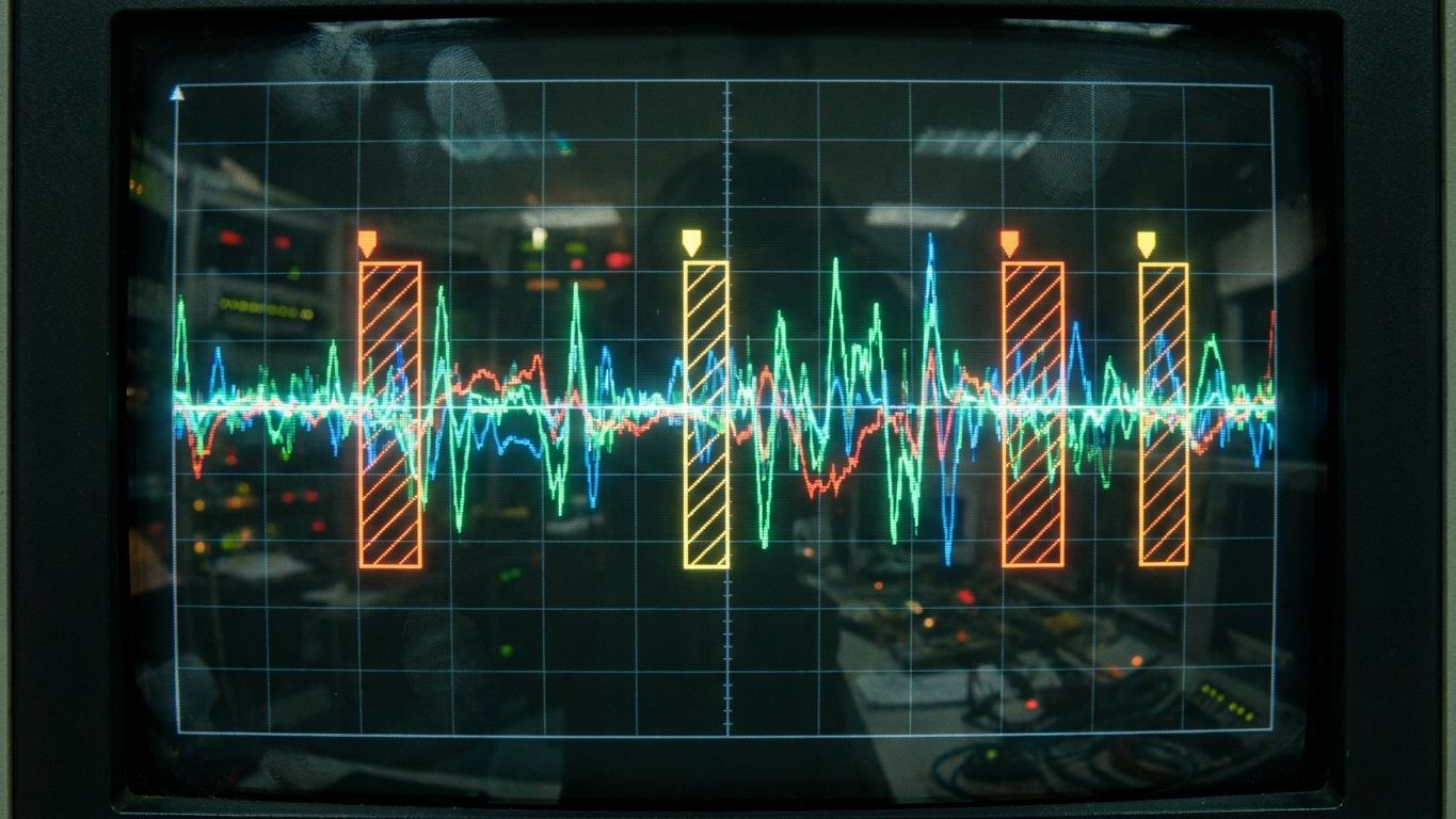
Phase 1 delivered a working velocity measurement system. Raw accelerometer data from the painting arm went through our signal processing pipeline: noise filtering, stroke segmentation, directional analysis, and velocity computation. The system could detect when painting velocity drifted outside acceptable bounds.

The problem: everything triggered drift alerts.

Operator pauses to reload paint canister. Velocity drops to zero. The system sees a massive velocity change and flags it.

Operator reverses direction at the edge of a panel. The deceleration-acceleration pattern looks like velocity instability.

Operator adjusts grip without stopping. Small velocity fluctuation that crosses the threshold.

Paint arm vibration during normal operation. High-frequency noise that occasionally pushes the computed velocity past the threshold.

Every one of these events was a real velocity change. The algorithm was right. But the operator wasn't painting poorly - they were painting normally. The system didn't understand the difference between bad painting and normal painting mechanics.

Technique 1: Hysteresis Thresholds

The Phase 1 system used a simple threshold: if velocity drops below X cm/s or exceeds Y cm/s, trigger an alert. One number. Binary decision.

The problem with single thresholds is boundary oscillation. An operator painting at 49.5 cm/s with a 50 cm/s minimum threshold will continuously trigger and un-trigger alerts as natural micro-variations push them above and below the line. The alert fires, clears, fires, clears - 20 times in 10 seconds.

Hysteresis uses two thresholds instead of one: an entry threshold and an exit threshold.

Entry threshold (trigger alert): Velocity drops below 45 cm/s. Exit threshold (clear alert): Velocity rises above 52 cm/s.

Once the velocity drops below 45, the alert stays active until velocity rises above 52. The gap between 45 and 52 is the hysteresis band. Small fluctuations inside this band don't trigger or clear alerts.

This eliminated approximately 35% of false positives. The oscillation-at-boundary problem disappeared entirely.

The tricky part was calibrating the band width. Too narrow and the oscillation problem returns. Too wide and real drift events get masked. We tested band widths from 3 cm/s to 15 cm/s against 200 hours of labeled factory data.

The optimal band width was 7 cm/s for the specific painting operations ProxControl monitored. This number is not universal. It depends on the typical velocity range, the sensor noise floor, and the acceptable drift tolerance for the specific coating process.

Technique 2: Debounce Windows

Even with hysteresis, brief events triggered alerts. An operator who paused for 0.3 seconds to shift their stance would cross the entry threshold, and because the pause was below the exit threshold for that brief moment, an alert fired.

Debounce adds a time requirement: the signal must stay past the threshold for a minimum duration before the alert triggers.

We implemented a 1.5-second debounce window. The velocity must remain below the entry threshold for 1.5 consecutive seconds before an alert fires. A 0.3-second pause doesn't count. A 0.8-second direction change doesn't count. Only sustained drift lasting 1.5+ seconds triggers an alert.

This eliminated another 30% of false positives. Brief transient events - pauses, direction changes, grip adjustments - almost always resolve within 1 second.

The debounce window interacts with hysteresis. The entry threshold sets where the alert triggers. The debounce sets how long it must persist. Together, they filter out both boundary oscillation and transient events.

Calibrating the debounce window required understanding the painting process. We asked: what is the shortest real drift event that operators should be alerted about? ProxControl's quality engineers said 2 seconds. Any drift shorter than 2 seconds doesn't affect coating quality measurably.

We set the debounce at 1.5 seconds to give a safety margin. A genuine drift event lasting 2 seconds triggers an alert at 1.5 seconds, giving the operator 0.5 seconds of warning before the coating quality degrades.

Technique 3: Movement Gating

The remaining false positives had a different pattern: they occurred during painting state transitions. Not during painting itself.

Loading paint: The arm is stationary. Velocity is zero. The system treats "zero velocity" as severe drift. Moving between panels: The arm moves quickly to the next panel without painting. Velocity is high but irrelevant - no paint is being applied. Calibration movements: Periodic arm recalibration involves specific motion patterns that look like erratic painting.

These aren't painting events at all. Alerting on them is like a speed camera ticketing a parked car.

Movement gating classifies the arm's state before evaluating velocity. We built a state machine with four states:

1. Painting - arm is moving within the painting zone with paint flow active 2. Transitioning - arm is moving between zones (high velocity, no paint flow) 3. Loading - arm is stationary or near-stationary (refueling) 4. Calibrating - arm is executing calibration patterns

Velocity drift alerts only fire during the Painting state. All other states are gated out.

Classifying the arm state required two additional signals beyond accelerometer data: paint flow rate (from the existing flow sensor) and position within the painting zone (from the existing position tracker). When paint flow rate is above zero and the arm is within the designated painting area, the state is Painting. Otherwise, it's one of the other three states.

Movement gating eliminated the remaining 26% of false positives. It was the simplest technique conceptually but required the most integration work because we needed data from sensors we hadn't used in Phase 1.

The Combined Pipeline

All three techniques run in series:

1. Raw velocity measurement (Phase 1 algorithm) 2. Movement gating: Is the arm in the Painting state? If no, suppress. 3. Hysteresis check: Has velocity crossed the entry threshold (or remained below the exit threshold if already alerting)? 4. Debounce check: Has the hysteresis condition persisted for 1.5+ seconds? 5. If all three checks pass: fire alert.

The order matters. Movement gating runs first because it's the cheapest filter - it eliminates 50%+ of evaluation windows without any signal processing. Hysteresis runs second. Debounce runs last because it requires tracking state over time, which is the most expensive operation.

Total processing latency for the combined pipeline: 12ms on the edge device. Well within the real-time requirement of 100ms maximum alert latency.

The Contrarian Take: We Should Have Built Movement Gating First

Looking back, we should have implemented movement gating in Phase 1. It was the single biggest improvement, and the concept is obvious in retrospect: don't evaluate painting quality when the operator isn't painting.

We didn't build it in Phase 1 because we were focused on the core velocity algorithm. The false positive problem seemed like a threshold tuning issue, not a state classification issue. We spent 2 weeks tuning thresholds before realizing the problem wasn't the thresholds at all.

The lesson: before optimizing a detection algorithm, make sure you're only evaluating the signal during relevant windows. Pre-filtering is often more impactful than post-filtering.

Calibration: The Ongoing Work

The three techniques solved the systemic false positive problem. But edge cases remained:

- Different paint viscosities produce different flow rates, which affect the movement gating thresholds - New operators paint differently from experienced operators (slower, more pauses) - Seasonal temperature changes affect paint viscosity and arm mechanics

We built a calibration mode that lets ProxControl's quality engineers adjust the hysteresis band, debounce window, and gating thresholds per paint type, per station, and per operator experience level. The calibration UI took 2 days to build. The algorithm work took 3 weeks.

This is typical for deep-tech projects: the algorithm is the hard part, the interface is the easy part.

Results

Before Phase 2: 47 false alerts per 8-hour shift. Operators ignored all alerts. After Phase 2: 4 false alerts per 8-hour shift. Operators respond to alerts within 5 seconds.

The 4 remaining false positives are edge cases we're still characterizing. Two are related to paint canister pressure drops that temporarily affect velocity. Two are sensor noise events that exceed the debounce window. We expect to reduce these to 1-2 per shift in the next calibration cycle.

The real metric isn't false positive count. It's operator trust. When the system cried wolf 47 times per shift, operators disabled it. At 4 times per shift, they keep it on and respond. A detection system that operators trust is infinitely more valuable than a detection system with 99.9% accuracy that no one uses.

Frequently Asked Questions

Can these techniques apply to other types of detection systems?

Yes. Hysteresis, debounce, and state gating are general-purpose false positive reduction techniques. We've used similar approaches in monitoring systems, anomaly detection, and IoT alerting. The specific threshold values change, but the architecture is transferable.

How much labeled data did you need to calibrate the system?

We used 200 hours of factory floor data labeled by ProxControl's quality engineers. About 40 hours were sufficient for initial calibration. The remaining 160 hours were used for validation and edge case discovery. If you're building a similar system, plan for at least 50 hours of labeled data.

What hardware runs the detection pipeline?

An industrial edge computing device (ARM-based, similar to a Raspberry Pi 4 in capability). The entire pipeline runs in under 12ms. We optimized for edge deployment because factory networks can't guarantee low-latency cloud connections. All processing is local.

How long did Phase 2 take?

4 weeks. Week 1 was analysis and approach selection. Weeks 2-3 were implementation and testing of all three techniques. Week 4 was factory validation, calibration UI, and documentation. Fixed-scope pricing at EUR 20k.

*Have an algorithm that's accurate but generates too many false positives? Book a 30-minute call and we'll discuss whether our approach applies to your detection problem. Or see our Deep-Tech Engineering service for details on how we handle algorithm projects.*